SlideShare una empresa de Scribd logo
1 de 8
Descargar para leer sin conexión
TALLER SERIE DE TAYLOR


                                 NORAIMA NAYARITH ZARATE GARCIA

                                                  COD. 2073173

                                              ING. DE PETROLEOS


1. Determine el n-ésimo polinomio de Taylor centrado en c de:

Serie de Taylor

                                                                                          f   xi
                                                                                               n
                                                                                                     
                                                       xi1  xi                                 xi1  xi 
                                                 f '' xi                      2                                           n
 f x     f xi  f ' xi                 x  xi                                      ...                                    R
    i1                                  i1        2!                                          n!


                           1
         a) f ( x)          ,          n=4,          c = 1 = xi
                           x

Solución

Hallamos cada una de las derivadas de la función dada y la evaluamos en xi=1:

               1                                                                    6
f ( xi )         1                                             f ' ' ' ( xi )       4
                                                                                          6
               xi                                                                   xi

                 1                                                                 24
f ' ( xi )         2
                       1                                       f IV ( xi )             24
                 xi                                                                 xi 5

                  2
f ' ' ( xi )       3
                      2
                 xi

Reemplazamos estos valores en la serie de Taylor y resolvemos para encontrar el
polinomio:

                                                                                                    
                                 2             2 (6)                3 24             4
 f x      1  (1) x  1          x 1                  x 1               x 1
    i 1               i 1      2! i 1             3! i 1               4! i 1

                                                                             
                                     2                3               4
 f x      1 x 1  x 1  x 1  x 1
    i 1          i 1       i 1           i 1            i 1
        xx
             i 1
         
   f x  2  x  x 2  2 x  1  x3  3 x 2  3 x  1  x 4  4 x 3  6 x 2  4 x  1
       f  x   x 4  5 x3  10 x 2  10 x  5
b) f ( x)  In( x) ,       n=4,       c = 1 = xi

Solución

Hallamos cada una de las derivadas de la función dada y la evaluamos en xi=1:


f ( xi )  In(1)  0                                                          2       2
                                                        f ' ' ' ( xi )           3
                                                                                     3 2
                                                                           ( xi )    1
               1 1
f ' ( xi )       1
               xi 1                                                            6      6
                                                        f IV ( xi )             4
                                                                                     4  6
                                                                            ( xi ) 1
                      1       1
f ' ' ( xi )            2
                             2  1
                   ( xi )    1

Reemplazando en la serie de Taylor f(x) y sus derivadas nos queda el siguiente
polinomio:

                                ( 1)            2 2            3 ( 6)             4
     f (x )  0  (x      1)        (x      1)  ( x      1)       (x      1)
         i 1       i 1          2!    i 1       3!  i 1         4!    i 1

                           1          2 1          3 1           4
     f (x )  (x      1)  ( x    1)  ( x    1)  ( x    1)
         i 1   i 1       2 i 1       3 i 1       4 i 1
               1
     f (x )     12 x  12  6( x  1) 2  4( x  1)3  3( x  1) 4 
         i 1 12  i 1           i 1          i 1         i 1    
               Hacemos la sustitución x  x
                                           i 1

               1 12 x  12  6 x  12 x  6 x  4  12 x  12 x  4  3 x  12 x 
                                 2            3          2                4      3
     f ( x)                                                                      
              12 18 x 2  12 x  3                                               
                    1
     f ( x)          3 x 4  16 x3  36 x 2  48 x  25
                   12                                    
                        x 4 4 x3   2        25
     f ( x)               3  3x  4 x 
                         3                  12

2. Para f(x) = arcsen (x)

a) Escribir el polinomio de MclaurinP3(x) para f(x).


Solución.
f (0)( xi 1 ) 2 f (0)( xi 1 )3        f n (0)( xi 1 ) n
 f ( x)  f ( xi 1 )  f (0)  f (0)( xi 1 )                                                       .. 
                                                                       2 !                3!                        n!
 Serie de de Mclaurin                       ( xi  0)


Hallamos cada una de las derivadas de la función dada y la evaluamos en xi=0:

                   1
f '( xi )                          f '(0)  1
                                    
                           2
                1  xi

                   xi
f ''( xi )                          f ''(0)  0
                                      
                            3
                       2
               (1  xi ) 2

                                                 2
                       1                  3 xi
f ''( xi )                                                  f '''(0)  1
                                                                
                               3                     5
                        2                    2
               (1  xi ) 2             (1  xi ) 2

Reemplazamos en la Serie de Mclaurin:

                                                                          (1)(( xi 1 )  0)3
                               f ( xi 1 )  0  (1)(( xi 1 )  0)  0 
                                                                                   3!
Reduciendo los términos                                      anteriores,      el    polinomio            de     Mclaurin           para
f(x)=arcsen(x), es:

                                                                                    ( xi1 )3
                                                     f ( xi1 )  ( xi1 ) 
                                                                                         6

     c) Completar la siguiente tabla para P3(x) y para f(x) (Utilizar radianes).

                                                     Valorverdadero  Valoraproximado
                                                                                           * 100
                                                                Valorverdadero

Los cálculos del error se realizan para cada uno de los valores de x de la Tabla 1:


 f ( x )  arcsen ( x )  arcsen ( 0.75)  0.8481
                                                     3                              3
                                        ( xi 1 )                        ( 0.75)
 f ( x )  ( xi 1 )                                    ( 0.75)                     0.8203
       i 1                                 6                                 6
           Valor verdadero  Valor aproximado        0.8481  ( 0.8203)
                                           *100                       *100  3.278
                     Valor verdadero                       0.8481
X             -0,75    -0,5             -0,25   0      0,25            0,5       0,75
   f(x)          -0,8481 -0,5236          -0,2527   0     0,2527         0,5236     0,8481
  P3(x)          -0,8203 -0,5208          -0,2526   0     0,2526         0,5208     0,8203
   %E             3,278   0,5348          0,03957   0    0,03957         0,5348      3,278
                                                                                       TABLA 1

c. Dibujar sus graficas en los mismos ejes coordenados.


3. Confirme la siguiente desigualdad con la ayuda de la calculadora y complete
la tabla para confirmar numéricamente.

                                   S  Ln ( x  1)  S
                                     2                              3


Siendo Sn la serie que aproxima la f(x) dada.

Solución

Aproximamos la función por medio de la serie de Mclaurin, donde xi=0

                1      1                                                 2        2
f '( xi )                1                       f '''( xi )                       2
              xi  1 0  1                                          ( xi  1)3 (0  1)3
                      1           1
f ''( xi )                             1
                 ( xi  1) 2
                               (0  1) 2


     Para S2 el polinomio es:
(1)(( xi 1 )  0) 2
f ( xi 1 )  ln(0  1)  (1)(( xi 1 )  0) 
                                                        2!
                         1
f ( xi 1 )  ( xi 1 )  ( xi 1 ) 2
                         2
    Para S3 el polinomio es:

                                                   (1)(( xi 1 )  0) 2 (2)(( xi 1 )  0)3
f ( xi 1 )  ln(0  1)  (1)(( xi 1 )  0)                          
                                                            2!                  3!
                         1             1
f ( xi 1 )  ( xi 1 )  ( xi 1 ) 2  ( xi 1 )3
                         2             3
    In (x+1)

f ( x)  ln( x  1)  ln(0.2  1)  0.1823

       S2
                                        2                               2
                            ( xi1 )                            (0.2)
f ( xi 1 )  ( xi 1 )                     (0.2)                         0.1800
                                2                                 2

       S3
                                        2                   2                          2               2
                            ( xi 1 )           ( xi 1 )                      (0.2)           (0.2)
f ( xi1 )  ( xi1 )                                          (0.2)                                   0.1826
                                2                     3                          2               3

Estos cálculos se realizan para cada uno de los valores de x en la Tabla 2:

         x             0,0                      0,2                0,4               0,6                   0,8          1

        S2                  0               0,1800               0,3200          0,4200              0,4800       0,5000

    In (x+1)                0               0,1823               0,3364          0,4700              0,5877           0,6931

        S3                  0               0,1826               0,3413          0,4920              0,6506       0,8333


Grafique y analice los resultados obtenidos

De acuerdo a los resultados obtenidos es claro que la función In (x+1) es mayor
que S3 pero menor que S2, por lo tanto la desigualdad no es correcta.
4. A partir de la serie de Taylor demostrar las expresiones de diferencia finita
regresiva y diferencia finita centrada.

Serie de Taylor:

                                                      f ' ' xi                        n 
    f xi 1   f xi   f ' xi xi 1  xi                 xi1  xi 2  ... f xi  xi1  xi n  R
                                                          2!                              n!


a. Diferencia finita regresiva:
Con la serie de Taylor truncamos en el segundo término, obteniendo:


                               f xi 1   f xi   f ' xi xi 1  xi 


Despejando la primera derivada:
                           (1)                     f  xi   f  xi 1 
                                    f '  xi  
                                                       xi 1  xi 
b. Diferencia finita centrada:
Para obtener la ecuación se requiere tener las series de diferencia finita regresiva
y diferencia finita progresiva.


Serie de Taylor para diferencias finitas progresivas:

                                       f ' ' xi  2 f ' ' ' xi  3 f IV xi  4         f n  xi  n
f xi 1   f xi   f ' xi h              h            h         h  ...             h  R
                                           2!             3!             4!                   n!

Con la serie de Taylor truncamos en el segundo término, obteniendo:
f xi 1   f xi   f ' xi xi 1  xi 
Ecuación para diferencias finitas progresivas, despejando la primera derivada:
                        (2)


Restando la ecuación (1) de (2), obtenemos:


Despejando la primera derivada:

                                                 f xi 1   f xi 1 
                                   f ' xi  
                                                   2( xi 1  xi 1 )

5. Usando los términos de la serie de Taylor, aproxime la función f(X)=cos(x) en
x0=π/3 con base en el valor de la función f y sus derivadas en el punto x1=π/4.
Empiece con solo el termino n=0 agregando sucesivamente un término hasta
que el error porcentual sea menor que la tolerancia, tomando 4 cifras
significativas.

Solución:

       Tolerancia

                                  E s   0.5x10²n  %      n = Cifras Significativas

                                                           n4
                                             E s   0.5x10² 4  %  5x105

       De acuerdo al enunciado:
                                                                            
                                   x                                  xi 
                                    i 1 3                                  4
           Hallamos las derivadas de la función:
                f  x   Cos  x                                     f ''  x   Cos  x 
                f '  x    Sen  x                                 f '''  x   Sen  x 

           Reemplazando tenemos:

                                                                    
                                                               Sen  
                                        Cos  x                 4   x     ...  f  xi   x   
                                                                2
                                                    
                                                                                   3        n                 n

 f  x   Cos    Sen   x                     x                                             
               4        4   4              2!      4      3!          4            n!          4
   Ahora empezamos a agregar término por término:

          
f    Cos    0.7071
  3       4

            Siguiente término:

                                        
                                   Cos               2
                           3        0.5220
f    Cos    Sen                         
  3       4        4  3 4     2!  3 4 

       Valornuevo  Valoranterior         0.5220  0.7071
a                               *100%                  *100%  35,5%
             Valornuevo                       0.5220


    Siguiente término:
                                                        
                                   Cos            2 Sen  
                           3          4        0.4999
                                                                          3

f    Cos    Sen                                          
  3       4        4  3 4     2!  3 4          3!  3 4 

       0.4999  0.5220
a                    *100%  4, 42%
           0.4999

Se continúa agregando términos hasta que           a   s como se muestra en la
tabla:


                  Términos             Resultado               εa(%)

                      1                  0.7071

                      2                 0.5220                 35.46

                      3                 0.4978                 4.86

                      4                 0,4999                 0.42

                      5                 0,5000                 0.02

                      6                 0.5000                   0


La aproximación usando el sexto término de la serie cumple con la tolerancia
exigida.

Más contenido relacionado

La actualidad más candente

Solucionparcial4 Cvusta2009 02
Solucionparcial4 Cvusta2009 02Solucionparcial4 Cvusta2009 02
Solucionparcial4 Cvusta2009 02guestf2c08f
 
Funciones a trozos
Funciones a trozosFunciones a trozos
Funciones a trozosguest01e453
 
Funciones exponenciales
Funciones exponencialesFunciones exponenciales
Funciones exponencialesCarlos Calle
 
Problemas1 Edo
Problemas1 EdoProblemas1 Edo
Problemas1 Edofvillena
 
Solucionquiz3 Cvusta2009 02
Solucionquiz3 Cvusta2009 02Solucionquiz3 Cvusta2009 02
Solucionquiz3 Cvusta2009 02guestf2c08f
 
Solucionquiz4 Cvusta2009 02
Solucionquiz4 Cvusta2009 02Solucionquiz4 Cvusta2009 02
Solucionquiz4 Cvusta2009 02guest4ea1e4
 
Trabajo final de matemáticas
Trabajo final de matemáticasTrabajo final de matemáticas
Trabajo final de matemáticasgabyart95
 
Ejercicios 5
Ejercicios 5Ejercicios 5
Ejercicios 5salgonsan
 
Caso Practico Funciones Exponenciales
Caso Practico Funciones ExponencialesCaso Practico Funciones Exponenciales
Caso Practico Funciones ExponencialesJudith Tornel
 
4 Temas Adicionales De La Derivada
4 Temas Adicionales De La Derivada4 Temas Adicionales De La Derivada
4 Temas Adicionales De La DerivadaERICK CONDE
 
Gráfica, curvas de nivel, límites
Gráfica, curvas de nivel, límitesGráfica, curvas de nivel, límites
Gráfica, curvas de nivel, límitesJIE MA ZHOU
 

La actualidad más candente (16)

Solucionparcial4 Cvusta2009 02
Solucionparcial4 Cvusta2009 02Solucionparcial4 Cvusta2009 02
Solucionparcial4 Cvusta2009 02
 
Funciones a trozos
Funciones a trozosFunciones a trozos
Funciones a trozos
 
Funciones exponenciales
Funciones exponencialesFunciones exponenciales
Funciones exponenciales
 
Problemas1 Edo
Problemas1 EdoProblemas1 Edo
Problemas1 Edo
 
Solucionquiz3 Cvusta2009 02
Solucionquiz3 Cvusta2009 02Solucionquiz3 Cvusta2009 02
Solucionquiz3 Cvusta2009 02
 
Fcd apuntes limites y continuidad
Fcd apuntes limites y continuidadFcd apuntes limites y continuidad
Fcd apuntes limites y continuidad
 
Solucionquiz4 Cvusta2009 02
Solucionquiz4 Cvusta2009 02Solucionquiz4 Cvusta2009 02
Solucionquiz4 Cvusta2009 02
 
Trabajo final de matemáticas
Trabajo final de matemáticasTrabajo final de matemáticas
Trabajo final de matemáticas
 
Ejercicios 5
Ejercicios 5Ejercicios 5
Ejercicios 5
 
Me02202 c
Me02202 cMe02202 c
Me02202 c
 
Ejercicios resueltos de derivadas
Ejercicios resueltos de derivadasEjercicios resueltos de derivadas
Ejercicios resueltos de derivadas
 
0. guia de repaso
0. guia de repaso0. guia de repaso
0. guia de repaso
 
Caso Practico Funciones Exponenciales
Caso Practico Funciones ExponencialesCaso Practico Funciones Exponenciales
Caso Practico Funciones Exponenciales
 
Funciones A Trozos
Funciones A TrozosFunciones A Trozos
Funciones A Trozos
 
4 Temas Adicionales De La Derivada
4 Temas Adicionales De La Derivada4 Temas Adicionales De La Derivada
4 Temas Adicionales De La Derivada
 
Gráfica, curvas de nivel, límites
Gráfica, curvas de nivel, límitesGráfica, curvas de nivel, límites
Gráfica, curvas de nivel, límites
 

Similar a Taller 1. serie de taylor

Reglas básicas de la derivación
Reglas básicas de la derivaciónReglas básicas de la derivación
Reglas básicas de la derivaciónjhbenito
 
7 aproximacion de funciones
7 aproximacion de funciones7 aproximacion de funciones
7 aproximacion de funcionesfenix1329
 
Soluciones funciones
Soluciones funcionesSoluciones funciones
Soluciones funcionesklorofila
 
Concepto de derivada
Concepto de derivadaConcepto de derivada
Concepto de derivadaITCN
 
Vértices y asíntotas (ejercicios)
Vértices y asíntotas (ejercicios)Vértices y asíntotas (ejercicios)
Vértices y asíntotas (ejercicios)Diannette Molinary
 
Soluciones limites
Soluciones limitesSoluciones limites
Soluciones limitesklorofila
 
Funcion cuadratica
Funcion cuadraticaFuncion cuadratica
Funcion cuadraticajpinedam
 
Solución trab extra clase brochure fun. expon
Solución trab extra clase brochure fun. exponSolución trab extra clase brochure fun. expon
Solución trab extra clase brochure fun. expondulcemrp
 
Guia ecuación cuadratica
Guia ecuación cuadraticaGuia ecuación cuadratica
Guia ecuación cuadraticasitayanis
 
Asíntotas y continuidad
Asíntotas y continuidadAsíntotas y continuidad
Asíntotas y continuidadmgarmon965
 
Ejercicios 6
Ejercicios 6Ejercicios 6
Ejercicios 6salgonsan
 
Taller de derivadas
Taller de derivadasTaller de derivadas
Taller de derivadasLenin Castro
 
funciones segundo medio
funciones segundo mediofunciones segundo medio
funciones segundo mediositayanis
 

Similar a Taller 1. serie de taylor (20)

Reglas básicas de la derivación
Reglas básicas de la derivaciónReglas básicas de la derivación
Reglas básicas de la derivación
 
Derivación
DerivaciónDerivación
Derivación
 
4 extremos
4 extremos4 extremos
4 extremos
 
7 aproximacion de funciones
7 aproximacion de funciones7 aproximacion de funciones
7 aproximacion de funciones
 
Soluciones funciones
Soluciones funcionesSoluciones funciones
Soluciones funciones
 
Concepto de derivada
Concepto de derivadaConcepto de derivada
Concepto de derivada
 
Vértices y asíntotas (ejercicios)
Vértices y asíntotas (ejercicios)Vértices y asíntotas (ejercicios)
Vértices y asíntotas (ejercicios)
 
Ejercicios derivadas
Ejercicios derivadasEjercicios derivadas
Ejercicios derivadas
 
Soluciones limites
Soluciones limitesSoluciones limites
Soluciones limites
 
Funcion cuadratica
Funcion cuadraticaFuncion cuadratica
Funcion cuadratica
 
Solución trab extra clase brochure fun. expon
Solución trab extra clase brochure fun. exponSolución trab extra clase brochure fun. expon
Solución trab extra clase brochure fun. expon
 
Guia ecuación cuadratica
Guia ecuación cuadraticaGuia ecuación cuadratica
Guia ecuación cuadratica
 
Tabla derivadas10 11
Tabla derivadas10 11Tabla derivadas10 11
Tabla derivadas10 11
 
Asíntotas y continuidad
Asíntotas y continuidadAsíntotas y continuidad
Asíntotas y continuidad
 
Ejercicios resueltos
Ejercicios resueltosEjercicios resueltos
Ejercicios resueltos
 
Ejercicios 6
Ejercicios 6Ejercicios 6
Ejercicios 6
 
Taller de derivadas
Taller de derivadasTaller de derivadas
Taller de derivadas
 
Taller 1 matemática ii limites
Taller 1 matemática ii limitesTaller 1 matemática ii limites
Taller 1 matemática ii limites
 
Funciones exponenciales
Funciones exponencialesFunciones exponenciales
Funciones exponenciales
 
funciones segundo medio
funciones segundo mediofunciones segundo medio
funciones segundo medio
 

Más de NORAIMA

Exercises
ExercisesExercises
ExercisesNORAIMA
 
Exercises
ExercisesExercises
ExercisesNORAIMA
 
Examples of iterative methods for the solution of
Examples of iterative methods for the solution ofExamples of iterative methods for the solution of
Examples of iterative methods for the solution ofNORAIMA
 
Iterative methods for the solution of systems of linear equations
Iterative methods for the solution of systems of linear equationsIterative methods for the solution of systems of linear equations
Iterative methods for the solution of systems of linear equationsNORAIMA
 
Iterative methods for the solution of systems of linear equations
Iterative methods for the solution of systems of linear equationsIterative methods for the solution of systems of linear equations
Iterative methods for the solution of systems of linear equationsNORAIMA
 
Iterative methods for the solution of systems of linear equations
Iterative methods for the solution of systems of linear equationsIterative methods for the solution of systems of linear equations
Iterative methods for the solution of systems of linear equationsNORAIMA
 
Iterative methods for the solution of systems of linear equations
Iterative methods for the solution of systems of linear equationsIterative methods for the solution of systems of linear equations
Iterative methods for the solution of systems of linear equationsNORAIMA
 
Examples of direct methods for the solution of systems of linear equations
Examples of direct methods for the solution of systems of linear equationsExamples of direct methods for the solution of systems of linear equations
Examples of direct methods for the solution of systems of linear equationsNORAIMA
 
Direct methods for the solution of systems of linear equations
Direct methods for the solution of systems of linear equationsDirect methods for the solution of systems of linear equations
Direct methods for the solution of systems of linear equationsNORAIMA
 
Matrices
MatricesMatrices
MatricesNORAIMA
 
Matrices
MatricesMatrices
MatricesNORAIMA
 
Matrices
MatricesMatrices
MatricesNORAIMA
 
Matrices
MatricesMatrices
MatricesNORAIMA
 
Examples methods of calculate roots of equation1
Examples   methods of calculate roots of equation1Examples   methods of calculate roots of equation1
Examples methods of calculate roots of equation1NORAIMA
 
Taller 1. serie de taylor
Taller 1. serie de taylorTaller 1. serie de taylor
Taller 1. serie de taylorNORAIMA
 
Methods of calculate roots of equations
Methods  of calculate  roots  of  equationsMethods  of calculate  roots  of  equations
Methods of calculate roots of equationsNORAIMA
 

Más de NORAIMA (16)

Exercises
ExercisesExercises
Exercises
 
Exercises
ExercisesExercises
Exercises
 
Examples of iterative methods for the solution of
Examples of iterative methods for the solution ofExamples of iterative methods for the solution of
Examples of iterative methods for the solution of
 
Iterative methods for the solution of systems of linear equations
Iterative methods for the solution of systems of linear equationsIterative methods for the solution of systems of linear equations
Iterative methods for the solution of systems of linear equations
 
Iterative methods for the solution of systems of linear equations
Iterative methods for the solution of systems of linear equationsIterative methods for the solution of systems of linear equations
Iterative methods for the solution of systems of linear equations
 
Iterative methods for the solution of systems of linear equations
Iterative methods for the solution of systems of linear equationsIterative methods for the solution of systems of linear equations
Iterative methods for the solution of systems of linear equations
 
Iterative methods for the solution of systems of linear equations
Iterative methods for the solution of systems of linear equationsIterative methods for the solution of systems of linear equations
Iterative methods for the solution of systems of linear equations
 
Examples of direct methods for the solution of systems of linear equations
Examples of direct methods for the solution of systems of linear equationsExamples of direct methods for the solution of systems of linear equations
Examples of direct methods for the solution of systems of linear equations
 
Direct methods for the solution of systems of linear equations
Direct methods for the solution of systems of linear equationsDirect methods for the solution of systems of linear equations
Direct methods for the solution of systems of linear equations
 
Matrices
MatricesMatrices
Matrices
 
Matrices
MatricesMatrices
Matrices
 
Matrices
MatricesMatrices
Matrices
 
Matrices
MatricesMatrices
Matrices
 
Examples methods of calculate roots of equation1
Examples   methods of calculate roots of equation1Examples   methods of calculate roots of equation1
Examples methods of calculate roots of equation1
 
Taller 1. serie de taylor
Taller 1. serie de taylorTaller 1. serie de taylor
Taller 1. serie de taylor
 
Methods of calculate roots of equations
Methods  of calculate  roots  of  equationsMethods  of calculate  roots  of  equations
Methods of calculate roots of equations
 

Taller 1. serie de taylor

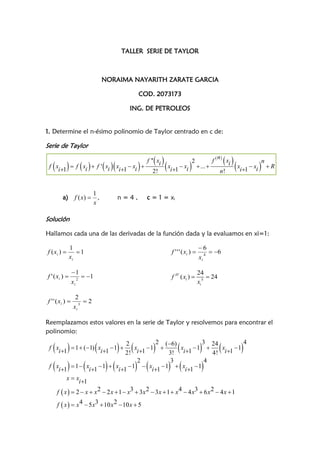
  • 1. TALLER SERIE DE TAYLOR NORAIMA NAYARITH ZARATE GARCIA COD. 2073173 ING. DE PETROLEOS 1. Determine el n-ésimo polinomio de Taylor centrado en c de: Serie de Taylor   f   xi n           xi1  xi   xi1  xi  f '' xi 2 n f x  f xi  f ' xi x  xi   ...  R i1 i1 2! n! 1 a) f ( x)  , n=4, c = 1 = xi x Solución Hallamos cada una de las derivadas de la función dada y la evaluamos en xi=1: 1 6 f ( xi )  1 f ' ' ' ( xi )  4  6 xi xi 1 24 f ' ( xi )  2  1 f IV ( xi )   24 xi xi 5 2 f ' ' ( xi )  3 2 xi Reemplazamos estos valores en la serie de Taylor y resolvemos para encontrar el polinomio:           2 2 (6) 3 24 4 f x  1  (1) x  1  x 1  x 1  x 1 i 1 i 1 2! i 1 3! i 1 4! i 1           2 3 4 f x  1 x 1  x 1  x 1  x 1 i 1 i 1 i 1 i 1 i 1 xx i 1   f x  2  x  x 2  2 x  1  x3  3 x 2  3 x  1  x 4  4 x 3  6 x 2  4 x  1 f  x   x 4  5 x3  10 x 2  10 x  5
  • 2. b) f ( x)  In( x) , n=4, c = 1 = xi Solución Hallamos cada una de las derivadas de la función dada y la evaluamos en xi=1: f ( xi )  In(1)  0 2 2 f ' ' ' ( xi )  3  3 2 ( xi ) 1 1 1 f ' ( xi )   1 xi 1 6 6 f IV ( xi )   4  4  6 ( xi ) 1 1 1 f ' ' ( xi )   2  2  1 ( xi ) 1 Reemplazando en la serie de Taylor f(x) y sus derivadas nos queda el siguiente polinomio: ( 1) 2 2 3 ( 6) 4 f (x )  0  (x  1)  (x  1)  ( x  1)  (x  1) i 1 i 1 2! i 1 3! i 1 4! i 1 1 2 1 3 1 4 f (x )  (x  1)  ( x  1)  ( x  1)  ( x  1) i 1 i 1 2 i 1 3 i 1 4 i 1 1 f (x )  12 x  12  6( x  1) 2  4( x  1)3  3( x  1) 4  i 1 12  i 1 i 1 i 1 i 1  Hacemos la sustitución x  x i 1 1 12 x  12  6 x  12 x  6 x  4  12 x  12 x  4  3 x  12 x  2 3 2 4 3 f ( x)    12 18 x 2  12 x  3  1 f ( x)  3 x 4  16 x3  36 x 2  48 x  25 12   x 4 4 x3 2 25 f ( x)    3  3x  4 x  3 12 2. Para f(x) = arcsen (x) a) Escribir el polinomio de MclaurinP3(x) para f(x). Solución.
  • 3. f (0)( xi 1 ) 2 f (0)( xi 1 )3 f n (0)( xi 1 ) n f ( x)  f ( xi 1 )  f (0)  f (0)( xi 1 )    ..  2 ! 3! n! Serie de de Mclaurin ( xi  0) Hallamos cada una de las derivadas de la función dada y la evaluamos en xi=0: 1 f '( xi )   f '(0)  1  2 1  xi xi f ''( xi )   f ''(0)  0  3 2 (1  xi ) 2 2 1 3 xi f ''( xi )     f '''(0)  1  3 5 2 2 (1  xi ) 2 (1  xi ) 2 Reemplazamos en la Serie de Mclaurin: (1)(( xi 1 )  0)3 f ( xi 1 )  0  (1)(( xi 1 )  0)  0  3! Reduciendo los términos anteriores, el polinomio de Mclaurin para f(x)=arcsen(x), es: ( xi1 )3 f ( xi1 )  ( xi1 )  6 c) Completar la siguiente tabla para P3(x) y para f(x) (Utilizar radianes). Valorverdadero  Valoraproximado  * 100 Valorverdadero Los cálculos del error se realizan para cada uno de los valores de x de la Tabla 1:  f ( x )  arcsen ( x )  arcsen ( 0.75)  0.8481 3 3 ( xi 1 ) ( 0.75)  f ( x )  ( xi 1 )   ( 0.75)   0.8203 i 1 6 6 Valor verdadero  Valor aproximado 0.8481  ( 0.8203)   *100  *100  3.278 Valor verdadero 0.8481
  • 4. X -0,75 -0,5 -0,25 0 0,25 0,5 0,75 f(x) -0,8481 -0,5236 -0,2527 0 0,2527 0,5236 0,8481 P3(x) -0,8203 -0,5208 -0,2526 0 0,2526 0,5208 0,8203 %E 3,278 0,5348 0,03957 0 0,03957 0,5348 3,278 TABLA 1 c. Dibujar sus graficas en los mismos ejes coordenados. 3. Confirme la siguiente desigualdad con la ayuda de la calculadora y complete la tabla para confirmar numéricamente. S  Ln ( x  1)  S 2 3 Siendo Sn la serie que aproxima la f(x) dada. Solución Aproximamos la función por medio de la serie de Mclaurin, donde xi=0 1 1 2 2 f '( xi )   1 f '''( xi )   2 xi  1 0  1 ( xi  1)3 (0  1)3 1 1 f ''( xi )     1 ( xi  1) 2 (0  1) 2  Para S2 el polinomio es:
  • 5. (1)(( xi 1 )  0) 2 f ( xi 1 )  ln(0  1)  (1)(( xi 1 )  0)  2! 1 f ( xi 1 )  ( xi 1 )  ( xi 1 ) 2 2  Para S3 el polinomio es: (1)(( xi 1 )  0) 2 (2)(( xi 1 )  0)3 f ( xi 1 )  ln(0  1)  (1)(( xi 1 )  0)   2! 3! 1 1 f ( xi 1 )  ( xi 1 )  ( xi 1 ) 2  ( xi 1 )3 2 3  In (x+1) f ( x)  ln( x  1)  ln(0.2  1)  0.1823  S2 2 2 ( xi1 ) (0.2) f ( xi 1 )  ( xi 1 )   (0.2)   0.1800 2 2  S3 2 2 2 2 ( xi 1 ) ( xi 1 ) (0.2) (0.2) f ( xi1 )  ( xi1 )    (0.2)    0.1826 2 3 2 3 Estos cálculos se realizan para cada uno de los valores de x en la Tabla 2: x 0,0 0,2 0,4 0,6 0,8 1 S2 0 0,1800 0,3200 0,4200 0,4800 0,5000 In (x+1) 0 0,1823 0,3364 0,4700 0,5877 0,6931 S3 0 0,1826 0,3413 0,4920 0,6506 0,8333 Grafique y analice los resultados obtenidos De acuerdo a los resultados obtenidos es claro que la función In (x+1) es mayor que S3 pero menor que S2, por lo tanto la desigualdad no es correcta.
  • 6. 4. A partir de la serie de Taylor demostrar las expresiones de diferencia finita regresiva y diferencia finita centrada. Serie de Taylor: f ' ' xi  n  f xi 1   f xi   f ' xi xi 1  xi   xi1  xi 2  ... f xi  xi1  xi n  R 2! n! a. Diferencia finita regresiva: Con la serie de Taylor truncamos en el segundo término, obteniendo: f xi 1   f xi   f ' xi xi 1  xi  Despejando la primera derivada: (1) f  xi   f  xi 1  f '  xi    xi 1  xi  b. Diferencia finita centrada: Para obtener la ecuación se requiere tener las series de diferencia finita regresiva y diferencia finita progresiva. Serie de Taylor para diferencias finitas progresivas: f ' ' xi  2 f ' ' ' xi  3 f IV xi  4 f n  xi  n f xi 1   f xi   f ' xi h   h  h  h  ... h  R 2! 3! 4! n! Con la serie de Taylor truncamos en el segundo término, obteniendo:
  • 7. f xi 1   f xi   f ' xi xi 1  xi  Ecuación para diferencias finitas progresivas, despejando la primera derivada: (2) Restando la ecuación (1) de (2), obtenemos: Despejando la primera derivada: f xi 1   f xi 1  f ' xi   2( xi 1  xi 1 ) 5. Usando los términos de la serie de Taylor, aproxime la función f(X)=cos(x) en x0=π/3 con base en el valor de la función f y sus derivadas en el punto x1=π/4. Empiece con solo el termino n=0 agregando sucesivamente un término hasta que el error porcentual sea menor que la tolerancia, tomando 4 cifras significativas. Solución: Tolerancia E s   0.5x10²n  % n = Cifras Significativas n4 E s   0.5x10² 4  %  5x105 De acuerdo al enunciado:   x  xi  i 1 3 4  Hallamos las derivadas de la función: f  x   Cos  x  f ''  x   Cos  x  f '  x    Sen  x  f '''  x   Sen  x   Reemplazando tenemos:   Sen     Cos  x    4   x     ...  f  xi   x    2       3 n n f  x   Cos    Sen   x     x       4  4  4 2!  4 3!  4 n!  4
  • 8. Ahora empezamos a agregar término por término:     f    Cos    0.7071 3 4  Siguiente término:   Cos   2            3        0.5220 f    Cos    Sen        3 4  4  3 4  2!  3 4  Valornuevo  Valoranterior 0.5220  0.7071 a  *100%  *100%  35,5% Valornuevo 0.5220  Siguiente término:     Cos   2 Sen              3      4        0.4999 3 f    Cos    Sen          3 4  4  3 4  2!  3 4  3!  3 4  0.4999  0.5220 a  *100%  4, 42% 0.4999 Se continúa agregando términos hasta que  a   s como se muestra en la tabla: Términos Resultado εa(%) 1 0.7071 2 0.5220 35.46 3 0.4978 4.86 4 0,4999 0.42 5 0,5000 0.02 6 0.5000 0 La aproximación usando el sexto término de la serie cumple con la tolerancia exigida.